# 植物空间转录组分析 1：Seurat 基本流程

# 植物空间转录组分析 2：STEEL+Seurat

# 前言

时隔半年的更新，这次的主题是单细胞 hdWGCNA 分析，文章刚刚被接收，目前在植物空间转录组已经有文章使用了该方法，基本的内容就是分 module 然后去看每个 module 的 hub 基因，或者做做 GO 富集之类的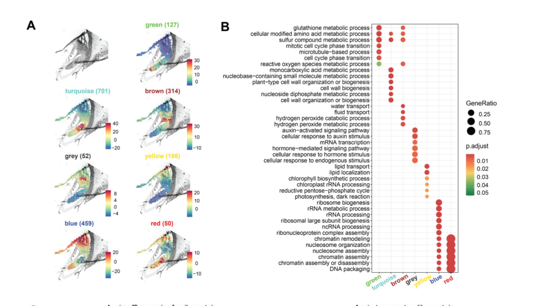
hdWGCNA

# R 包安装以及数据准备

本次分析还是以兰花的空间转录组为基础，具体的数据参考以前的推文

	# install BiocManager
	install.packages("BiocManager")

	# install Bioconductor core packages
	BiocManager::install()

	# install additional packages:
	install.packages(c("Seurat", "WGCNA", "igraph", "devtools"))

	devtools::install_github('smorabit/hdWGCNA', ref='dev')

大家可能会因为网络问题无法下载，我直接将压缩包发给大家

	## 数据准备
	## 将 spot 坐标信息加到 metadata 中
	# make a dataframe containing the image coordinates for each sample
	image_df <- do.call (rbind, lapply (names (orc1_new@images), function (x){
	orc1_new@images [[x]]@coordinates
	}))

	# merge the image_df with the Seurat metadata
	new_meta <- merge (orc1_new@meta.data, image_df, by='row.names')

	# fix the row ordering to match the original seurat object
	rownames (new_meta) <- new_meta$Row.names
	ix <- match (as.character (colnames (orc1_new)), as.character (rownames (new_meta)))
	new_meta <- new_meta [ix,]

	# add the new metadata to the seurat object
	orc1_new@meta.data <- new_meta

# 构建 metaspots

	## Here we set up the data for hdWGCNA and run MetaspotsByGroups.

	subdata <- subset(orc1_new, idents = c(19,21,37,38,39,40))
	subdata <- SCTransform(subdata, assay = "Spatial", return.only.var.genes = FALSE, verbose = FALSE)
	subdata <- RunPCA(subdata, features = VariableFeatures(subdata))

	subdata <- SetupForWGCNA(
	subdata,
	features = VariableFeatures(subdata),
	wgcna_name = "SCT"
	)


	subdata <- MetacellsByGroups(
	seurat_obj = subdata,
	group.by = c("seurat_clusters"),
	k = 5,
	max_shared= 10,
	min_cells = 6,
	reduction = 'pca',
	ident.group = 'seurat_clusters',
	slot = 'scale.data',
	assay = 'SCT'
	)
	m_obj <- GetMetacellObject(subdata)
	m_obj
	An object of class Seurat
	14006 features across 180 samples within 1 assay
	Active assay: SCT (14006 features, 0 variable features)

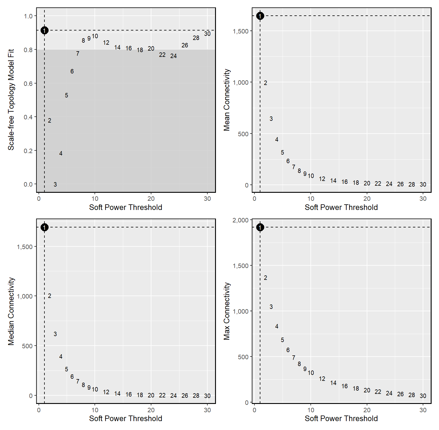
这里需要注意，一般空间分析推荐使用的是 MetaspotsByGroups 函数，我尝试了一遍 softpower 只有 1，module 只有两个，所以又使用了 MetacellsByGroups 函数尝试。

# 共表达网络分析

	# set up the expression matrix, set group.by and group_name to NULL to include all spots
	subdata <- SetDatExpr(
	subdata,
	group.by=NULL,
	group_name = NULL
	)

	# test different soft power thresholds
	subdata <- TestSoftPowers(subdata)
	plot_list <- PlotSoftPowers(subdata)

	wrap_plots(plot_list, ncol=2)

softpowers

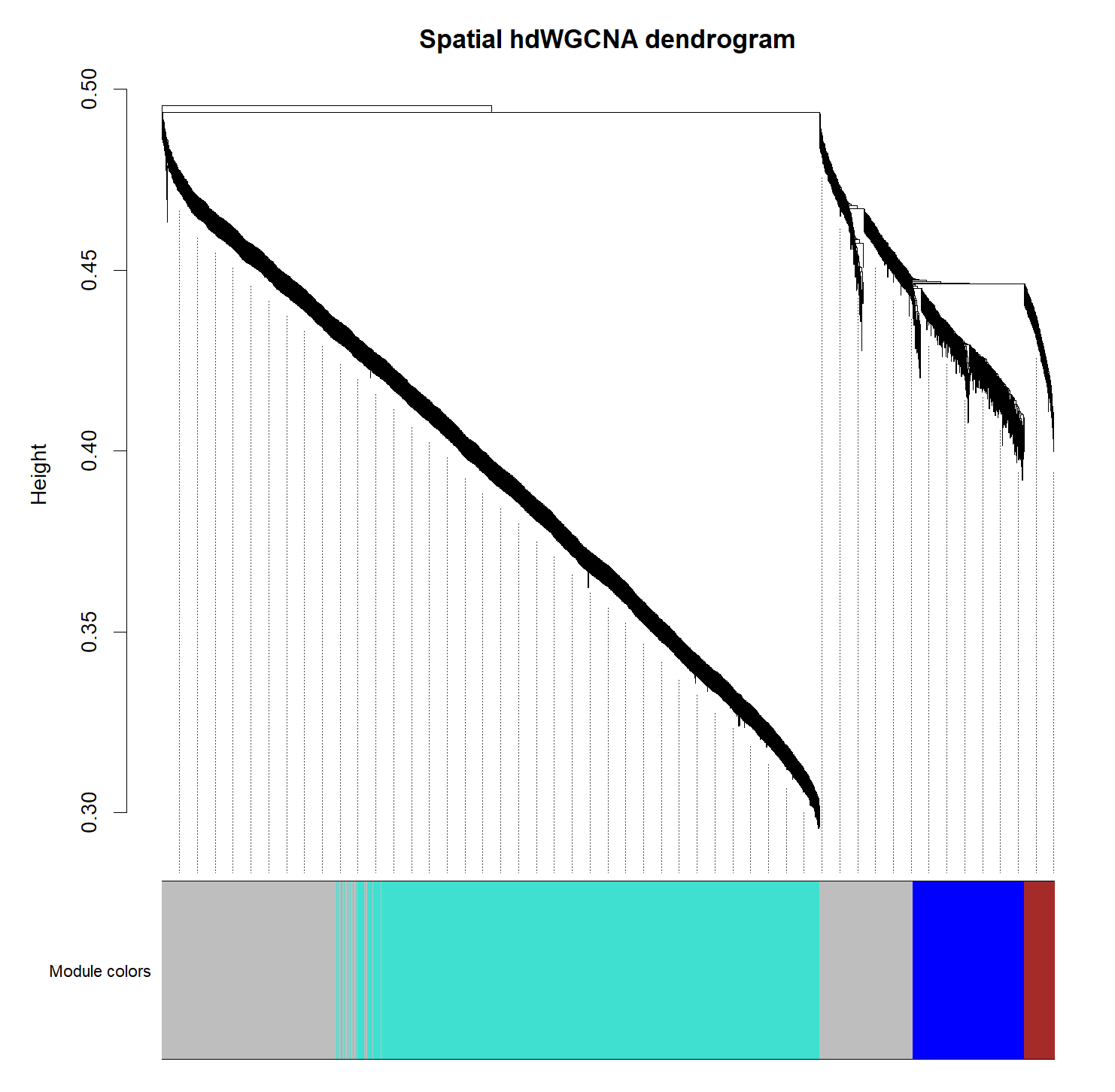
# construct co-expression network:
subdata <- ConstructNetwork(
  subdata,
  soft_power = 1,
  tom_name='test',
  overwrite_tom=TRUE
)

# plot the dendrogram
PlotDendrogram(subdata, main='Spatial hdWGCNA dendrogram')

dendrogram

# compute module eigengenes

	subdata <- ModuleEigengenes(subdata)
	subdata <- ModuleConnectivity(subdata)

	modules <- GetModules(subdata) %>% subset(module != 'grey')
	head(modules[,1:3])

	gene_name module color
	PAXXG297280 PAXXG297280 turquoise turquoise
	PAXXG074500 PAXXG074500 blue blue
	PAXXG239080 PAXXG239080 turquoise turquoise
	PAXXG067750 PAXXG067750 turquoise turquoise
	PAXXG327430 PAXXG327430 turquoise turquoise
	PAXXG311150 PAXXG311150 blue blue

模块数目比较少也是正常的

# Data visualization

	tom<-GetTOM(subdata)
	##Data visualization
	##Here we visualize module eigengenes using the Seurat functions DotPlot and SpatialFeaturePlot.
	##For network visualization, please refer to the Network visualization tutorial.
	# get module eigengenes and gene-module assignment tables
	MEs <- GetMEs(subdata)
	modules <- GetModules(subdata)
	mods <- levels(modules$module)

	write.table(file="modules.xls",modules,row.names = F,sep="\t")
	# plot with Seurat's DotPlot function
	p <- DotPlot(subdata, features=mods, group.by = 'seurat_clusters', dot.min=0.1)

	# flip the x/y axes, rotate the axis labels, and change color scheme:
	p <- p +
	coord_flip() +
	RotatedAxis() +
	scale_color_gradient2(high='red', mid='grey95', low='blue') +
	xlab('') + ylab('')

	p



	p <- SpatialFeaturePlot(
	subdata,
	features = mods,
	ncol = 4,
	pt.size.factor = 3.5
	)

	p

{.gallery data-height="300"}
分别用两种方法展示

# module network plots

分为两种，一种每个模块的 hubgene，一种是全部模块的 hubgene

	## Individual module network plots
	ModuleNetworkPlot(subdata,
	plot_size = c(10, 10),
	vertex.label.cex = 0.6
	)

	hub_df <- GetHubGenes(subdata, n_hubs = 25)
	write.table(file="hub_df.xls",hub_df,row.names = F,sep="\t")

	## hubgene network


	HubGeneNetworkPlot(
	subdata,
	n_hubs = 4, n_other=6,
	edge_prop = 0.75,
	mods = 'all',
	hub.vertex.size = 4,
	other.vertex.size = 1,
	edge.alpha = 0.5
	)

# 总结

目前只是初步上手，其实这个方法主要的目的还是根据表达对基因进行聚类，再加个功能富集可能会更好，后续还有 UMAP to co-expression networks 流程，但因为我在做的时候效果比较差所以没放。