# 前言
目前我的课题是植物方面的单细胞测序,所以打算选择植物类的单细胞测序数据进行复现,目前选择了王佳伟老师的《A Single-Cell RNA Sequencing Profiles the Developmental Landscape of Arabidopsis Root》,希望能够得到好的结果
# 原始数据的下载
首先下载测序数据
prefetch SRR8485805 -O wang/ | |
fastq-dump --split-files SRR8485805 | |
mv SRR8485805_1.fastq data/WT_S1_L001_I1_001.fastq | |
mv SRR8485805_2.fastq data/WT_S1_L001_R1_001.fastq | |
mv SRR8485805_3.fastq data/WT_S1_L001_R2_001.fastq |
下载基因组与注释文件,需要注意文献中基因组使用的是 TAIR10,注释文件是 Araport11。
将 gff 转为 gtf 文件
gffread Araport11.gff3 -T -o Araport11.gtf |
# cellranger 进行比对
下载 cellranger2.2 版本
curl -o cellranger-2.2.0.tar.gz "https://cf.10xgenomics.com/releases/cell-exp/cellranger-2.2.0.tar.gz?Expires=1603141363&Policy=eyJTdGF0ZW1lbnQiOlt7IlJlc291cmNlIjoiaHR0cHM6Ly9jZi4xMHhnZW5vbWljcy5jb20vcmVsZWFzZXMvY2VsbC1leHAvY2VsbHJhbmdlci0yLjIuMC50YXIuZ3oiLCJDb25kaXRpb24iOnsiRGF0ZUxlc3NUaGFuIjp7IkFXUzpFcG9jaFRpbWUiOjE2MDMxNDEzNjN9fX1dfQ__&Signature=en6P4Wedmwc2aSEitfKsQp2PITVYKgRPZdzR-fEmjBl4R9yQY5QBQY05--1v8AzRD9WqfoCnddSzFvngrlwxzeCJtFyfHLa2a7ONnUT6NtrzU6RkIj1jwXpaN4NpixnCbEF-Ubj9UZX63W1rEreM0AMNdWiVneGx4bcTajl1KRWaoTNS970DSJ1wrw0g70JFQ0BAltou-qPAeZpD9Xe9EM35EdWRT6eFq~zOaCMRLTxlBjZaMItyDRH~Qecz-B5tLWcAjCKfy4o2hAWTopRRpy93LVV-x1ykxCiHpej5AuAODvUx0V73rZOkRlijcpA5d1rHV~eEdPiM1uoCOJMiSw__&Key-Pair-Id=APKAI7S6A5RYOXBWRPDA" | |
tar -zxvf cellranger-2.2.0.tar.gz |
建立索引并比对
/datadisk02/ScRNAseq_data/cellranger-2.2.0/cellranger mkref --genome=ref --fasta=TAIR10.fa --genes=Araport11.gtf | |
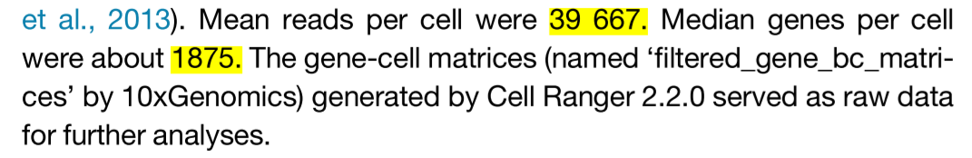
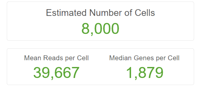
/datadisk02/ScRNAseq_data/cellranger-2.2.0/cellranger count --id=WANG --transcriptome=ref --fastqs=data/ --sample=WT --force-cells=8000 |
比对结果还是可以的,与原文献中差距很小
# 使用 Seurat 对数据进行分析
文献中使用到的 Seurat 为 V3 版本,要注意 cellrangeV2 在 filtered_gene_bc_matrices 生成的文件是 genes、barcodes 以及 matrix,但 Seurat 识别的是 features,我们需要自行对 genes 文件改名
cd WANG/outs/filtered_gene_bc_matrices/ref | |
gzip genes.tsv | |
gzip matrix.mtx | |
gzip barcodes.tsv | |
mv genes.tsv.gz features.tsv.gz |
# 创建 Seurat 对象
library (Seurat) | |
library (dplyr) | |
library (ggplot2) | |
library (magrittr) | |
library (gtools) | |
library (stringr) | |
library (Matrix) | |
library (tidyverse) | |
library (patchwork) | |
setwd ("D://data/ScRNAcode/wang/") | |
##=======================1. 创建 Seurat 对象 ======================== | |
dir <- 'filtered_gene_bc_matrices/ref/' | |
counts <- Read10X (dir) | |
wang = CreateSeuratObject (counts, project = "zxz", min.cells=3, min.features = 200) | |
dim (wang) | |
[1] 23228 8000 |
# 数据质控与标准化
##=======================2. 数据质控与标准化 ================================ | |
##dir.create ('QC') | |
## 提取线粒体基因 | |
wang [["percent.mt"]] <- PercentageFeatureSet (wang, pattern='^ATMG') | |
violin <- VlnPlot (wang, | |
features = c ("nFeature_RNA", "nCount_RNA", "percent.mt"), | |
pt.size = 0.1, #不需要显示点,可以设置 pt.size = 0 | |
ncol = 3) | |
ggsave ("QC/vlnplot-before-qc.pdf", plot = violin, width = 15, height = 6) | |
ggsave ("QC/vlnplot-before-qc.png", plot = violin, width = 15, height = 6) | |
plot1 <- FeatureScatter (wang, feature1 = "nCount_RNA", feature2 = "percent.mt") | |
plot2 <- FeatureScatter (wang, feature1 = "nCount_RNA", feature2 = "nFeature_RNA") | |
pearplot <- CombinePlots (plots = list (plot1, plot2), nrow=1, legend="none") | |
ggsave ("QC/pearplot-before-qc.pdf", plot = pearplot, width = 12, height = 5) | |
ggsave ("QC/pearplot-before-qc.png", plot = pearplot, width = 12, height = 5) | |
## 设置质控标准 | |
wang<-subset (wang,subset=nFeature_RNA>500 & nFeature_RNA<5000 &percent.mt<0.5) | |
dim (wang) | |
[1] 23228 7626 | |
## 绘制质量控制后的图 | |
violin <-VlnPlot (wang, | |
features = c ("nFeature_RNA", "nCount_RNA", "percent.mt"), | |
pt.size = 0.1, | |
ncol = 3) | |
ggsave ("QC/vlnplot-after-qc.pdf", plot = violin, width = 15, height = 6) | |
ggsave ("QC/vlnplot-after-qc.png", plot = violin, width = 15, height = 6) | |
## 基因表达量标准化 | |
## 它的作用是让测序数据量不同的细胞的基因表达量具有可比性。计算公式如下: | |
## 标准化后基因表达量 = log1p(10000 * 基因 counts / 细胞总 counts) | |
wang <- NormalizeData (wang, normalization.method = "LogNormalize", scale.factor = 10000) |
质控后细胞数目为 7626,基因数为 23228,原文献中两者的数据分别是 7695 与 23161
# 数据降维与聚类
##=======================3. 数据降维与聚类 ================================== | |
## 寻找高变基因 | |
## dir.create ("cluster") | |
wang <- FindVariableFeatures (wang,mean.cutoff=c (0.0125,3),dispersion.cutoff =c (1.5,Inf) ) | |
top10 <- head (VariableFeatures (wang), 10) | |
plot1 <- VariableFeaturePlot (wang) | |
plot2 <- LabelPoints (plot = plot1, points = top10, repel = TRUE, size=2.5) | |
plot <- CombinePlots (plots = list (plot1, plot2),legend="bottom") | |
## 横坐标是某基因在所有细胞中的平均表达值,纵坐标是此基因的方差。 | |
## 红色的点是被选中的高变基因,黑色的点是未被选中的基因,变异程度最高的 10 个基因在如图中标注了基因名称。 | |
ggsave ("cluster/VariableFeatures.pdf", plot = plot, width = 8, height = 6) | |
ggsave ("cluster/VariableFeatures.png", plot = plot, width = 8, height = 6) | |
## 数据缩放 | |
scale.genes <- rownames (wang) | |
wang <- ScaleData (wang, features = scale.genes) | |
## PCA 降维并提取主成分 | |
wang <- RunPCA (wang, features = VariableFeatures (wang),npcs = 100) | |
plot1 <- DimPlot (wang, reduction = "pca") | |
plot2 <- ElbowPlot (wang, ndims=40, reduction="pca") | |
plotc <- plot1+plot2 | |
ggsave ("cluster/pca.pdf", plot = plotc, width = 8, height = 4) | |
ggsave ("cluster/pca.png", plot = plotc, width = 8, height = 4) | |
## 细胞聚类 | |
## 此步利用 细胞 - PC 值 矩阵计算细胞之间的距离, | |
## 然后利用距离矩阵来聚类。其中有两个参数需要人工选择, | |
## 第一个是 FindNeighbors () 函数中的 dims 参数,需要指定哪些 pc 轴用于分析,选择依据是之前介绍的 cluster/pca.png 文件中的右图。 | |
## 第二个是 FindClusters () 函数中的 resolution 参数,需要指定 0.1-1.0 之间的一个数值,用于决定 clusters 的相对数量,数值越大 cluters 越多。 | |
wang <- FindNeighbors (object = wang, dims = 1:100) | |
wang <- FindClusters (object = wang, resolution = 1.0) | |
table (wang@meta.data$seurat_clusters) | |
## 非线性降维 | |
## tsne | |
wang <- RunTSNE (wang, dims =1:40) | |
embed_tsne <- Embeddings (wang, 'tsne') | |
write.csv (embed_tsne,'cluster/embed_tsne_new.csv') | |
plot1 = DimPlot (wang, reduction = "tsne" ,label = "T", pt.size = 1,label.size = 4) | |
ggsave ("cluster/tSNE_cluster.pdf", plot = plot1, width = 8, height = 7) | |
ggsave ("cluster/tSNE_cluster.png", plot = plot1, width = 8, height = 7) | |
## UMAP' | |
wang <- RunUMAP (wang,n.neighbors = 30,metric = 'correlation',min.dist = 0.3,dims = 1:40) | |
embed_umap <- Embeddings (wang, 'umap') | |
write.csv (embed_umap,'cluster/embed_umap_new.csv') | |
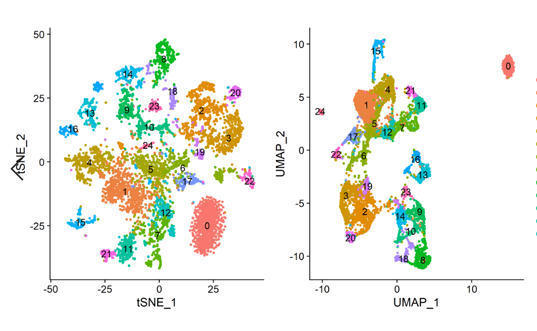
plot2 = DimPlot (wang, reduction = "umap",label = "T", pt.size = 1,label.size = 4) | |
ggsave ("cluster/UMAP_cluster_new.pdf", plot = plot2, width = 8, height = 7) | |
ggsave ("cluster/UMAP_cluster_new.png", plot = plot2, width = 8, height = 7) |
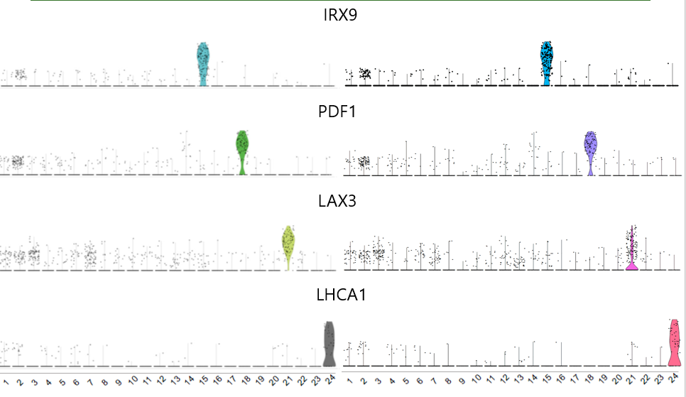
结果是有区别的,我的聚类比原文献中要多一个,而且数字不对应,所以我要用文献中列出的某些基因的小提琴图确定我的聚类
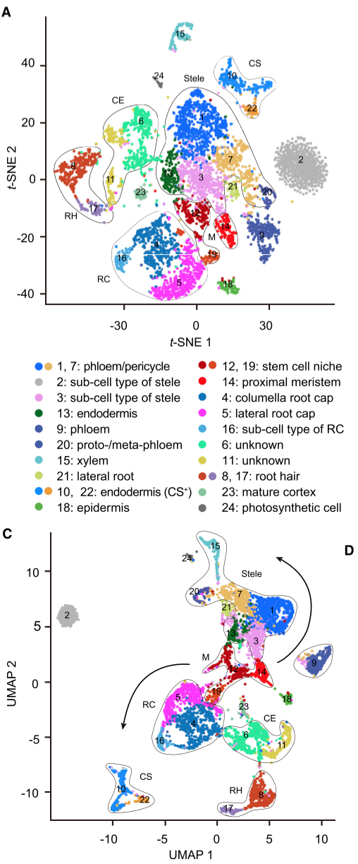
# 根据文献对应自己数据聚类
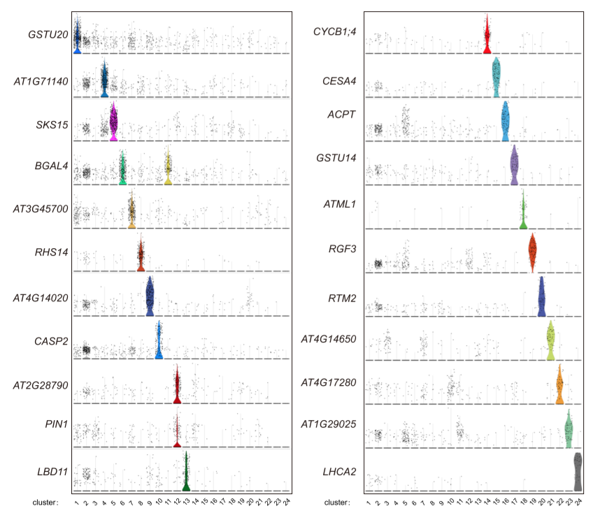
原文献中有所有聚类的特异基因,所以我根据列出的基因去匹配我的聚类结果
##==============================5. 修改聚类标号 ===================== | |
## 修改聚类号重新做图 | |
new.cluster.ids<-c ("2",'1','4','5','13','3','12','21','8','6','11', | |
'9','7','10','6','15','22','14','17','19','16', | |
'20','18','23','24') | |
names (new.cluster.ids) <- levels (wang) | |
wang <- RenameIdents (wang, new.cluster.ids) | |
Idents (wang)<-factor (Idents (wang),levels=mixedsort (levels (Idents (wang)))) | |
wang <- RunTSNE (wang, dims =1:40) | |
embed_tsne <- Embeddings (wang, 'tsne') | |
write.csv (embed_tsne,'cluster/embed_tsne-new.csv') | |
plot1 = DimPlot (wang, reduction = "tsne" ,label = "T", pt.size = 1,label.size = 4) | |
ggsave ("cluster/tSNE_cluster-new.pdf", plot = plot1, width = 8, height = 7) | |
ggsave ("cluster/tSNE_cluster-new.png", plot = plot1, width = 8, height = 7) | |
## UMAP | |
wang <- RunUMAP (wang,n.neighbors = 30,metric = 'correlation',min.dist = 0.3,dims = 1:40) | |
embed_umap <- Embeddings (wang, 'umap') | |
write.csv (embed_umap,'cluster/embed_umap-new.csv') | |
plot2 = DimPlot (wang, reduction = "umap",label = "T", pt.size = 1,label.size = 4) | |
ggsave ("cluster/UMAP_cluster.pdf", plot = plot2, width = 8, height = 7) | |
ggsave ("cluster/UMAP_cluster.png", plot = plot2, width = 8, height = 7) |
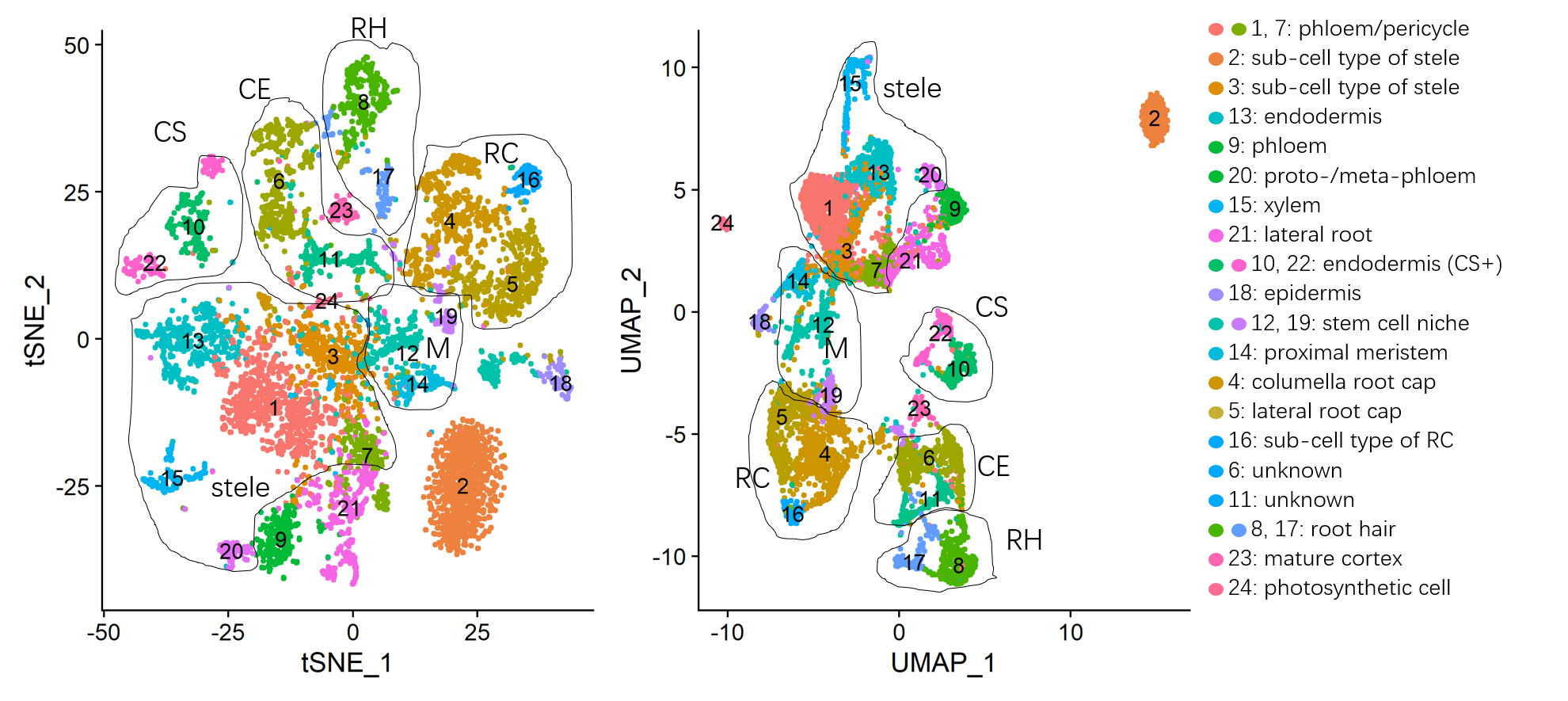
修改之后的聚类结果
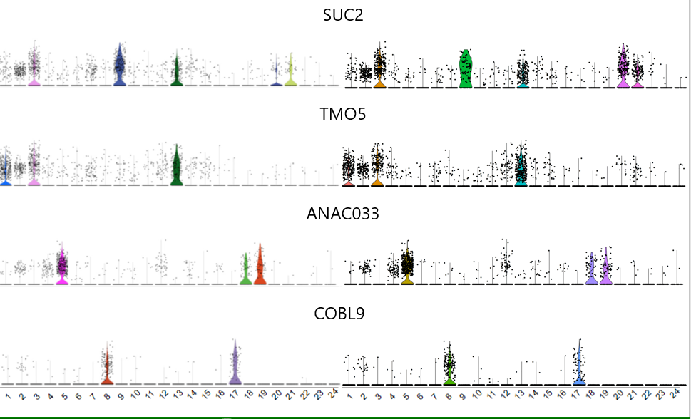
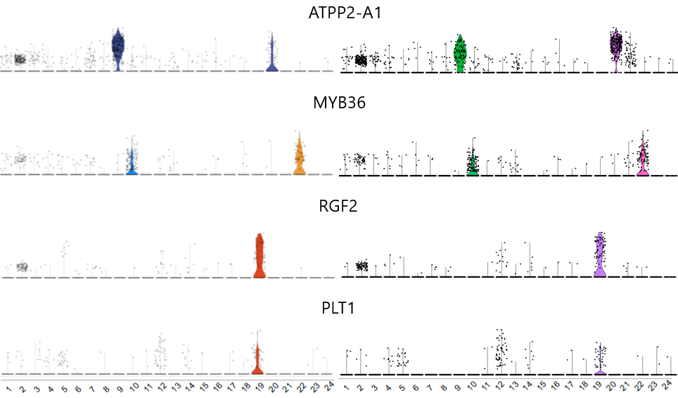
一些基因的小提琴图对应效果
# 结语
对于这次的数据重复,基本符合预期结果,和文章的结果有点差距,需要自己进一步研究问题出在哪里,下一次将继续这篇文献的数据复现,主要是伪时间分析,目前的数据与代码我已上传 github